Today's hot topic: Loudspeaker design basics, part 5
Product: Loudspeaker drive units
Price: musical resolution
Humble scribe: Mark Wheeler - TNT UK
Typed: Spring 2009
OK plebs: stand by your beds! We've gotta shape up and ship out 'cos there's work to do.
"Not those infernal noisy power tools again?" Demand plebs, stage left;
The only power tool you'll need today is a pocket calculator, reassures the old speaker builder
We already considered the basic purpose of our loudspeakers in part 1 and the generalities of choosing and using drive units in part 4, so now we are ready to scrutinise those catalogues with our calculators in our hands.
"What?" Demand plebs, from stage left, "Surely we're going to use software to model bass response from T/S
parameters; surely the old fool isn't going to make us manually calculate spot frequencies and plot them on graph paper? Doesn't
the old fool know what century we're in?"
"Well," replieth the ancient one, "bass alignment isn't the only thing we can derive from specs, and is possibly one of
the least audible decisions we'll make at the design stage assuming we choose an alignment somewhere between Bessel and Butterworth.
Furthermore, sometimes the tedious detailed activity of manually drawing out graphs is more informative as it makes us stop and think:
it certainly works for load lines when juicing up a valve (tube), but that's another story."
We all remember from school that F=ma, don't we?
In a moving coil loudspeaker the F (force) is a product of the magnet strength and the juice in the voice coil in the
magnet gap. Unsurprisingly this is usually shown in the Thiele Small drive unit parameters as BL product.
So substituting this in our well known equation we get BL=ma.
So rearranging we now know that we can calculate motor acceleration from a=BL/m, or rather Γ=BL/m.
That wasn't difficult was it? a (acceleration), expressed as Γ (uppercase gamma), will obviously be measured in metres per second (speed) per second (rate of change of speed, aka acceleration), commonly written as ms^-2 (metres per second squared). However, this is acceleration factor, (hence being expressed as 'Γ' rather than 'a') so, like any other factor in physics or engineering, it is specific, i.e. context dependent. Therefore the unit of its context needs to be included, which is the 1A current applied to generate each packet of acceleration.
The m (mass) in question is the mass of the moving parts of the loudspeaker. We know we're talking about "moving coil" loudspeakers, so obviously the coil is one moving part. The next moving part is the cone that is glued to the front rim of the voice coil former, so we have to add this mass to that of the coil. The final moving mass is that part of the rear spider suspension that moves (the suspension that centres the voice-coil in the pole piece gap) and the part of cone front edge surround that moves. Sadly this may not be linear as the amount of corrugated suspension that moves with the cone during a very small excursion may not be the same as that during a large excursion. However for the purposes of drive unit Parameter measurement it is common to assume the small excursion situation and specification sheets are likely to reflect this. Fortunately we home constructors do not need to worry our pretty little heads about these niceties as the manufacturers have done all that for us when they prepared the table of Thiele Small Parameters. However manufacturers foolishly often express moving mass in grammes, and unless the Systeme Internationale has changed the accepted definitions, mass should always be expressed in kg, remember to check and if necessary convert by exp-3.
So there we have it. Look at the the data sheet and type the BL product figure into your calculator. Now type the division sign.
Now type the mass in kg. Now press the equals button.
The figure you now have, usually between 100 and 1000 theoretically defines the maximum acceleration of the coil and cone in the drive
unit under consideration. Superficially this ought to define the upper bandwidth limit of the drive unit, but for various reasons it may
not. It is when the relationship between these two figures is not congruent that we begin to derive insights into the driver behaviour
that might help us decide whether an unauditioned drive unit should be accepted or rejected from our shortlist for that new project.
How does this help us, the home designer/constructor?
|
|
When this has been described elsewhere (Wheeler 1999 p34-36) there have been counter arguments that this calculation merely describes the theoretical bandwidth limit of a driver. Indeed this would be the case with rigid cone drivers designed to work below their first break-up frequency, such as anodised aluminium cones. In such cases the defined resolution of the driver must be higher than the corner frequency of the low-pass filter in the crossover. However, in the past flexible annular rings were commonly used on paper cones (and still are in guitar amp speakers) to introduce controlled cone break-up and extend bandwidth and nowadays many cone drivers rely on carefully controlled cone break-up to extend the upper bandwidth by exponential profiles of modern plastics thus also reducing the moving mass with rising frequency.
How does that work? demand plebs, stage left, "The old fool's contradicting himself again"
Well, replieth ye old one, if the designer can develop a cone profile & material combination (basically by balancing mass
and flexibility - that's why you should have listened when teacher talked about Young's Modulus) that allows the cone to flex
in proportion to frequency, the measured output of the cone will hang in there to a higher frequency that would have been the case
with a rigid cone. A secondary advantage is that the reduced cone area at higher frequencies will result in wider dispersion (better
polar response) than from the full diameter of the cone if moving like a piston.
"Wow!" scream plebs, stage left, "We don't get something for nothing very often in audio,
this sounds too good to be true!"
Indeed its sound would be surprisingly good if it were true, but while it most certainly is a sound it is not a 'true'
sound. It is inevitably distorted from the original.
The further the cone flexure is used to extend the response above the motor assembly
resolution, the more distorted the output becomes compared with the original signal at those frequencies. The character of the
distortion from cone flexure is behind the sonic signature of different cone materials (onto which is added the dynamics of cone
termination and adhesives). Controlled cone flexure is a very useful device in driver design, enabling drive units to cover
much wider bandwidths than would otherwise be possible. This means less drivers per system. This also means less crossover points.
That means simpler filters, and we already know the disadvantages of
complicated crossover filters
For home constructors designing systems from scratch it is worthwhile knowing the theoretical resolving power of a drive unit that is not yet necessarily relying on distortion to grab a freebie octave more. If we have the T/S data from four 200mm drive units in front of us, from which we are attempting to select a bass-mid unit for our next project, we might wish to know how their potential in that critical mid-band where human and instrumental expression is most concentrated and where our hearing is, by no coincidence, most sensitive.
Let us say our tweeter suspension resonance of Q=1 is just above 1kHz. We wish to avoid that high Q=1 (anything above Q=0.7 should be an anathema in high quality loudspeaker design) so will prefer to align the 3rd order (18dB per octave) crossover comfortably above 2kHz to avoid the resonance peak creating output at near passband levels an octave below at 1kHz. We look at the graphs from our various woofer manufacturers to see which one will allow the low-pass section to reach over 2kHz. All four might look like they reach 3kHz before falling away gracefully, some more spiky than others.
We might assume the more spiky looking responses indicate that those drive units are distorting more than the smoother looking graphs. We might guess that this implies that the rougher curves indicate that the designers of those drive units are relying more one controlled cone break-up than the smooth looking ones. No, NO, NO! It merely suggests that the smooth looking ones were printed out with a lower pen-speed or faster chart-speed, or both. Unless that data is present along the bottom, the curves are meaningless in all respects except general trends. Equally, unless they are all taken from a drive unit flush mounted in an IEC standard dimensioned baffle they are useless for comparison anyway.
So we examine at the curves from our four likely looking 200mm drivers and they all have similar looking trends above 200Hz. They all exhibit the gently rising response engendered by voice coil inductance and reasonably sized magnet assemblies. None have any glitches in the impedance curves suggesting sudden unexpected phase shifts (other than the expected one on the fs) caused by resonance. Now, dear reader, it is time to get the calculators out.
|
|
It is clear that there can be a wide distribution of values that are neither dominated by magnet size nor cone mass in four 200mm drivers from the same manufacturer (not a range available at present, nor a manufacturer who supplies the retail market). These drivers are all designed to meet different OEM needs, at different price=points, with different fs (free air resonance), different cone materials, different sensitivities and with different loading. None is a better drive unit than the others. All are application specific, and the designer hope each on is the best compromise for that application.
However, the result of designing each of these to meet their target specification is that when the lights go green driver 3 accelerates away 3 times faster than driver 4. If we want undistorted bandwidth into the upper midrange driver 3 looks like ti might have an immediate advantage at the business end. A glance at the other T/S parameters suggest driver 4 will go much deeper at the bas end so we might choose it for another design with a low pass crossover point below 1kHz, it only struggles along to -6dB at 3kHz via a massive peak at 1.7kHz.
The only way to gather evidence for any hypothesis is to test it (Wheeler 1999). As it happens, in 1993 I had the opportunity to set up a test. I had two pairs of 200mm drivers from the same manufacturer, using the same chassis baskets but different magnets and voice coils. Both were destined to be bass-midrange units, but in very different alignments and cabinet sizes. Driver A offered Γ=650ms^-2.A^-1 and driver B offered Γ=390ms^-2.A^-1. In order to minimise the effects of their (dramatic) bass response differences I used an active crossover to bandwidth limit them from 200Hz to 2kHz. A 250mm driver handled the lower octaves and a 25mm anodised aluminium dome (working a little too low for complete comfort) handled the top end decade. The crossover was used to equalise sensitivity and frequency response was close enough between the drivers to require no tailoring. Both drivers were matched with a Zobel network across their terminals. Tests were with a single speaker fed with summed stereo (often mis-termed mono).
With a wide variety of programme material the results were consistent. Driver A sounded consistently more detailed and more transparent. Driver A also sounded more dynamic, but this will be the subject of a later article. It was as if driver B were subject to some compression. Driver B has a lower BL product as a result of a longer voice coil for sealed enclosure applications and also much higher power handling due to a larger 40mm voice coil diameter. Extra length or extra diameter will reduce BL product with a given magnet size and driver B gets both. In this test driver A was consistently judged superior subjectively.
As an aside, when mounted in their designed applications, driver B produced much deeper more tuneful bass in its Bessel alignment sealed big box (hence 2nd order Q~0.577) than the more sensitive smaller box reflex loaded driver A, whose short 25mm voice coil needed a QB3 alignment to keep it in the gap. You do not get something for nothing and this phenomenon may have contributed to the increasing popularity of the two-&-a-half way floorstander in recent years.
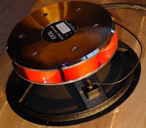
![[hammering at my heart]](../jpg/hammer_driver.jpg)
It is possible to predict more than bass alignment from Thiele Small parameters. It's possible to develop hypotheses (make educated guesses) about performance near the top of drive unit bandwidth. These guesses are based on the capabilities of the motor system to respond to the signal rather than clever engineering of cone flexure to extend the apparent response. As home constructors we seldom get the opportunity to listen to raw drivers before purchase so any extra judgements we can extrapolate from the facts provided are a help in making a shortlist.
|
© Copyright 2009 Mark Wheeler - www.tnt-audio.com